44 excel scatter chart labels

Present your data in a scatter chart or a line chart 09.01.2007 · Often referred to as an xy chart, a scatter chart never displays categories on the horizontal axis. A scatter chart always has two value axes to show one set of numerical data along a horizontal (value) axis and another set of numerical values along a vertical (value) axis. The chart displays points at the intersection of an x and y numerical ... Excel Scatter Chart with Labels - Super User Move the button down and out of the way of your data if you have more than a few columns. Paste your data in on top of the film data. Create scatter plots by selecting two column at a time and insert scatter (plot). Clicking on the button, which will add labels. Easy.

Add Custom Labels to x-y Scatter plot in Excel Step 1: Select the Data, INSERT -> Recommended Charts -> Scatter chart (3 rd chart will be scatter chart) Let the plotted scatter chart be Step 2: Click the + symbol and add data labels by clicking it as shown below Step 3: Now we need to add the flavor names to the label. Now right click on the label and click format data labels.

Excel scatter chart labels

Scatter chart excel - JulianMeesha Select the data you want to plot in the scatter chart. Add Labels to Scatter Plot Excel Data Points. To create or make Scatter Plots in Excel you have to follow below step by step process Select all the cells that contain data. Following are the steps to insert a Scatter chart-. The data points are represented as individual dots and are. How to display text labels in the X-axis of scatter chart in Excel? Display text labels in X-axis of scatter chart. Actually, there is no way that can display text labels in the X-axis of scatter chart in Excel, but we can create a line chart and make it look like a scatter chart. 1. Select the data you use, and click Insert > Insert Line & Area Chart > Line with Markers to select a line chart. See screenshot: Creating Scatter Plot with Marker Labels - Microsoft Community Right click any data point and click 'Add data labels and Excel will pick one of the columns you used to create the chart. Right click one of these data labels and click 'Format data labels' and in the context menu that pops up select 'Value from cells' and select the column of names and click OK.

Excel scatter chart labels. How to Add Axis Labels in Excel Charts - Step-by-Step (2022) - Spreadsheeto Left-click the Excel chart. 2. Click the plus button in the upper right corner of the chart. 3. Click Axis Titles to put a checkmark in the axis title checkbox. This will display axis titles. 4. Click the added axis title text box to write your axis label. excel - How to label scatterplot points by name? - Stack Overflow This is what you want to do in a scatter plot: right click on your data point select "Format Data Labels" (note you may have to add data labels first) put a check mark in "Values from Cells" click on "select range" and select your range of labels you want on the points UPDATE: Colouring Individual Labels Create a Pareto Chart in Excel (In Easy Steps) - Excel Easy If you don't have Excel 2016 or later, simply create a Pareto chart by combining a column chart and a line graph. This method works with all versions of Excel. 1. First, select a number in column B. 2. Next, sort your data in descending order. On the Data tab, in the Sort & Filter group, click ZA. 3. Calculate the cumulative count. Enter the ... Improve your X Y Scatter Chart with custom data labels - Get Digital Help The first 3 steps tell you how to build a scatter chart. Select cell range B3:C11 Go to tab "Insert" Press with left mouse button on the "scatter" button Press with right mouse button on on a chart dot and press with left mouse button on on "Add Data Labels"

How to use a macro to add labels to data points in an xy scatter chart ... In Microsoft Office Excel 2007, follow these steps: Click the Insert tab, click Scatter in the Charts group, and then select a type. On the Design tab, click Move Chart in the Location group, click New sheet , and then click OK. Press ALT+F11 to start the Visual Basic Editor. On the Insert menu, click Module. How To Create Scatter Chart in Excel? - EDUCBA To apply the scatter chart by using the above figure, follow the below-mentioned steps as follows. Step 1 - First, select the X and Y columns as shown below. Step 2 - Go to the Insert menu and select the Scatter Chart. Step 3 - Click on the down arrow so that we will get the list of scatter chart list which is shown below. Multiple Time Series in an Excel Chart - Peltier Tech 12.08.2016 · Any of the formatting described here applies to all of these chart types. XY Scatter charts are different: X axes behave like Y axes. I could write a book just on this subject. Displaying Multiple Time Series in An Excel Chart. The usual problem here is that data comes from different places. While the data may span a similar range of dates, the ... How to Create a Scatter Plot in Excel with 3 Variables ... - ExcelDemy Step-02: Generate Scatter Plot. Generating a scatter plot diagram with your data points can help you to determine the potential relationship between them. To generate a scatter chart follow the steps: Steps: At first, select Column B, Column C, and Column D. Then, click the Insert tab and go to the Insert Scatter option, and select Scatter.

Prevent Overlapping Data Labels in Excel Charts - Peltier Tech Hi Jon, I know the above comment says you cant imagine handing XY charts but if there is any update on this i really need it :) i have a scatterplot/bubble chart and can have say 4 different labels that all refer to one position on a bubble chart e.g. say X=10, Y=20 can have 4 different text labels (e.g. short quotes). Change the format of data labels in a chart To get there, after adding your data labels, select the data label to format, and then click Chart Elements > Data Labels > More Options. To go to the appropriate area, click one of the four icons ( Fill & Line, Effects, Size & Properties ( Layout & Properties in Outlook or Word), or Label Options) shown here. Excel Chart Vertical Axis Text Labels • My Online Training Hub Apr 14, 2015 · Note how the vertical axis has 0 to 5, this is because I've used these values to map to the text axis labels as you can see in the Excel workbook if you've downloaded it. Step 2: Sneaky Bar Chart. Now comes the Sneaky Bar Chart; we know that a bar chart has text labels on the vertical axis like this: Excel: labels on a scatter chart, read from array - Stack Overflow You will get the desired results by following the steps below: Step 1: Click on the Chart Step 2: Select the Design Tab in Ribbon Bar (Note: "Design Tab" appears only when the Chart is selected) Step 3: Click on "Select Data" feature in the Design Tab as shown in Screen Shot 1 Step 4: Click on Edit Button as shown in Screen Shot 2 Step 5: Change...

Combine pie and xy scatter charts - Advanced Excel Charting Example

Find, label and highlight a certain data point in Excel scatter graph To let your users know which exactly data point is highlighted in your scatter chart, you can add a label to it. Here's how: Click on the highlighted data point to select it. Click the Chart Elements button. Select the Data Labels box and choose where to position the label.

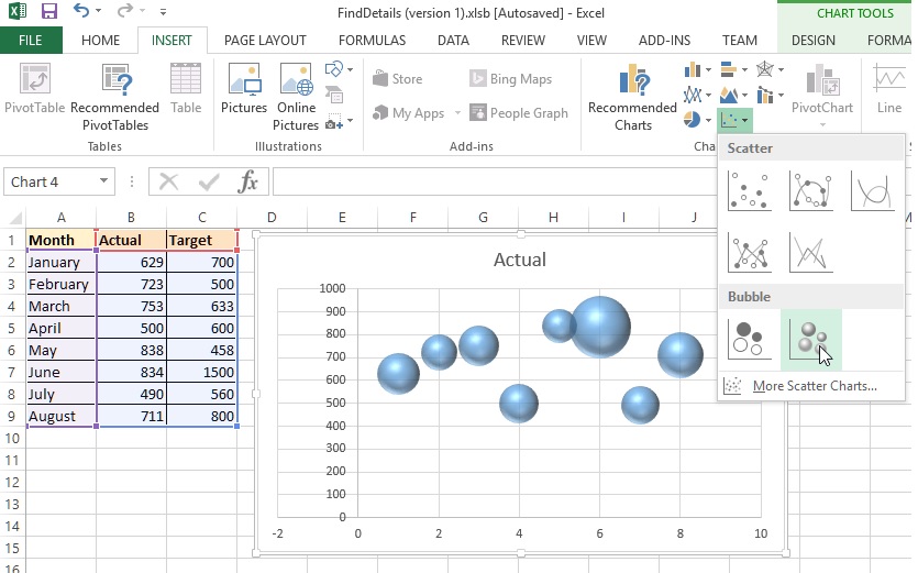
2D & 3D Bubble chart in Excel - Tech Funda

How to Add Labels to Scatterplot Points in Excel - Statology Step 1: Create the Data First, let's create the following dataset that shows (X, Y) coordinates for eight different groups: Step 2: Create the Scatterplot Next, highlight the cells in the range B2:C9. Then, click the Insert tab along the top ribbon and click the Insert Scatter (X,Y) option in the Charts group. The following scatterplot will appear:

How to create a Scatterplot with Dynamic Reference Lines in Excel

How do I set labels for each point of a scatter chart? Click one of the data points on the chart. Chart Tools. Layout contextual tab. Labels group. Click on the drop down arrow to the right of:- Data Labels Make your choice. If my comments have helped please vote as helpful. Thanks. Report abuse Was this reply helpful? Yes No

Excel Training 101: Create an X Y Scatter Chart with Data Labels

How to create a scatter plot in Excel with 3 variables Making a scatter plot. Heres how easy it is to make one: For sure, you too would be able to make one in 5 seconds after this tutorial. Kasper Langmann, Co-founder of Spreadsheeto. Lets break what just happened: 1st click: Select the two columns with the data. In our example, its B3:C14.

Multiple Series in One Excel Chart - Peltier Tech Blog

How to add text labels on Excel scatter chart axis Stepps to add text labels on Excel scatter chart axis 1. Firstly it is not straightforward. Excel scatter chart does not group data by text. Create a numerical representation for each category like this. By visualizing both numerical columns, it works as suspected. The scatter chart groups data points. 2. Secondly, create two additional columns.

How to Make Scatter Charts in Excel - Uses | Features

How to Add X and Y Axis Labels in Excel (2 Easy Methods) 2. Using Excel Chart Element Button to Add Axis Labels. In this second method, we will add the X and Y axis labels in Excel by Chart Element Button. In this case, we will label both the horizontal and vertical axis at the same time. The steps are: Steps: Firstly, select the graph. Secondly, click on the Chart Elements option and press Axis Titles.

Advanced Excel - круговые диаграммы - CoderLessons.com

How to Find, Highlight, and Label a Data Point in Excel Scatter Plot ... By default, the data labels are the y-coordinates. Step 3: Right-click on any of the data labels. A drop-down appears. Click on the Format Data Labels… option. Step 4: Format Data Labels dialogue box appears. Under the Label Options, check the box Value from Cells . Step 5: Data Label Range dialogue-box appears.

Share :