41 pie chart excel labels

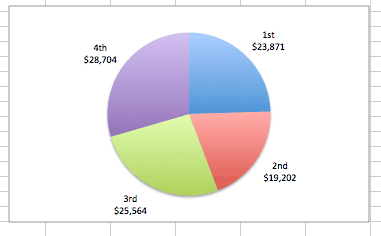
Excel 2010 pie chart data labels in case of "Best Fit" Based on my tested in Excel 2010, the data labels in the "Inside" or "Outside" is based on the data source. If the gap between the data is big, the data labels and leader lines is "outside" the chart. And if the gap between the data is small, the data labels and leader lines is "inside" the chart. Regards, George Zhao. TechNet Community Support. Is there a way to change the order of Data Labels? Replied on April 4, 2018. Hi Keith, I got your meaning. Please try to double click the the part of the label value, and choose the one you want to show to change the order. Thanks, Rena. -----------------------. * Beware of scammers posting fake support numbers here. * Once complete conversation about this topic, kindly Mark and Vote any ...

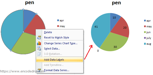
How to Create and Format a Pie Chart in Excel - Lifewire Select the plot area of the pie chart. Right-click the chart. Select Add Data Labels . Select Add Data Labels. In this example, the sales for each cookie is added to the slices of the pie chart. Change Colors When a chart is created in Excel, or whenever an existing chart is selected, two additional tabs are added to the ribbon.

Pie chart excel labels

excel - Positioning data labels in pie chart - Stack Overflow Positioning data labels in pie chart. I'm trying to format some charts I have, using VBA. To get started I recorded a macro of me doing what I wanted, to have an idea of what methods I'd want etc. The recorded macro looks like this - I'm including the whole thing, though the line to pay attention to is Selection.Position = xlLabelPositionCenter. How to Make a Pie Chart in Excel & Add Rich Data Labels to The Chart! Creating and formatting the Pie Chart 1) Select the data. 2) Go to Insert> Charts> click on the drop-down arrow next to Pie Chart and under 2-D Pie, select the Pie Chart, shown below. 3) Chang the chart title to Breakdown of Errors Made During the Match, by clicking on it and typing the new title. Microsoft Excel Tutorials: Add Data Labels to a Pie Chart You should get the following menu: From the menu, select Add Data Labels. New data labels will then appear on your chart: The values are in percentages in Excel 2007, however. To change this, right click your chart again. From the menu, select Format Data Labels: When you click Format Data Labels , you should get a dialogue box.

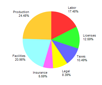
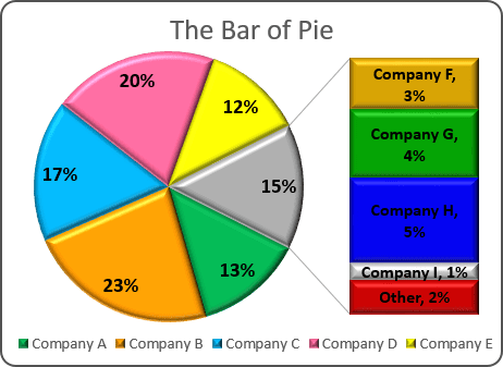
Pie chart excel labels. Explode or expand a pie chart - support.microsoft.com Pie-of-pie and bar-of-pie charts make it easier to see small slices of a pie chart. These chart types separate the smaller slices from the main pie chart and display them in a secondary pie—or stacked bar chart. In the example below, a pie-of-pie chart adds a secondary pie to show the three smallest slices. Compare a normal pie chart before: How to Create a Pie Chart in Excel | Smartsheet To create a pie chart in Excel 2016, add your data set to a worksheet and highlight it. Then click the Insert tab, and click the dropdown menu next to the image of a pie chart. Select the chart type you want to use and the chosen chart will appear on the worksheet with the data you selected. Pie Chart in Excel - Inserting, Formatting, Filters, Data Labels Right click on the Data Labels on the chart. Click on Format Data Labels option. Consequently, this will open up the Format Data Labels pane on the right of the excel worksheet. Mark the Category Name, Percentage and Legend Key. Also mark the labels position at Outside End. This is how the chark looks. Formatting the Chart Background, Chart Styles Chart Legend / Data Labels In Pie Chart | MrExcel Message Board Add the data labels. Then, right click on any data label to select all the data labels for that series and select Format Data Labels... From the Label Options tab, in the Label Contains section, select the 'Series Name' checkbox. The above applies to Excel 2007. Excel 2003 supports the same capability though the dialog box choices may be different.

How to Create a Family Tree Chart in Excel, Word, Numbers ... Step 1: Create a New Spreadsheet. Launch a new Excel document by clicking the start button, and then click on Microsoft Office to select Microsoft Excel Templates.Once all that is done, click File from the menu and click New to select a template to create a family tree. Pie Chart - legend missing one category (edited to include spreadsheet ... Right click in the chart and press "Select data source". Make sure that the range for "Horizontal (category) axis labels" includes all the labels you want to be included. PS: I'm working on a Mac, so your screens may look a bit different. But you should be able to find the horizontal axis settings as describe above. Multiple Data Labels on a Pie Chart | MrExcel Message Board So I have a table with 8 rows and 3 columns. This table includes: Column 1 - shipment name. Column 2 - shipment cost. Column 3 - shipment weight. I have created a pie chart from this table, which covers the first two columns. Displayed next to each slice is a label with the shipment name, shipment cost, and percent share of the pie. Only Display Some Labels On Pie Chart - Excel Help Forum Only Display Some Labels On Pie Chart. I have a pie chart that contains over 50 categories (Yes, I know pie charts shouldn't be used for that many things) but I want to only display labels for maybe the top 5 values or any label with a value >10. This is because there are a few standout values but I want all the other values to remain in the ...

Everything You Need to Know About Pie Chart in Excel How to Make a Pie Chart in Excel. Start with selecting your data in Excel. If you include data labels in your selection, Excel will automatically assign them to each column and generate the chart. Go to the INSERT tab in the Ribbon and click on the Pie Chart icon to see the pie chart types. Click on the desired chart to insert. excel - How to not display labels in pie chart that are 0% - Stack Overflow Generate a new column with the following formula: =IF (B2=0,"",A2) Then right click on the labels and choose "Format Data Labels". Check "Value From Cells", choosing the column with the formula and percentage of the Label Options. Under Label Options -> Number -> Category, choose "Custom". Under Format Code, enter the following: How to Customize Your Excel Pivot Chart Data Labels - dummies The Data Labels command on the Design tab's Add Chart Element menu in Excel allows you to label data markers with values from your pivot table. When you click the command button, Excel displays a menu with commands corresponding to locations for the data labels: None, Center, Left, Right, Above, and Below. None signifies that no data labels should be added to the chart and Show signifies ... Free Pie Chart Maker - Make Your Own Pie Chart | Visme To use the pie chart maker, click on the data icon in the menu on the left. Enter the Graph Engine by clicking the icon of two charts. Choose the pie chart option and add your data to the pie chart creator, either by hand or by importing an Excel or Google sheet.

Chart Data Labels in PowerPoint 2013 | Windows PowerPoint Tutorials

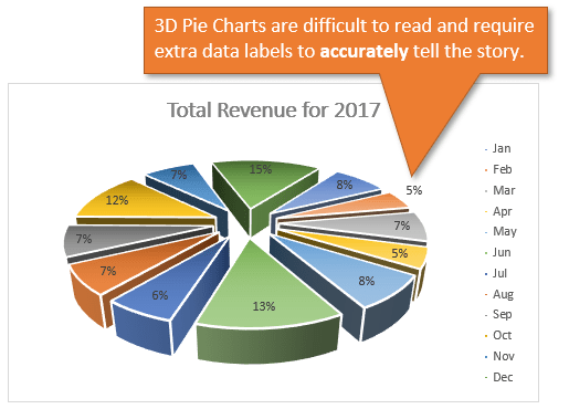
Pie Chart Best Fit Labels Overlapping - VBA Fix - Microsoft Tech Community I created attached Pie chart in Excel with 31 points and all labels are readable and perfectly placed. It is created from few clicks without VBA using data visualization tool in Excel. Data Visualization Tool For Excel Data Visualization Tool For Google Sheets It has auto cluttering effect to adjust according to your data size.

How to Create a Pie Chart in Excel | Smartsheet

How to display leader lines in pie chart in Excel? - ExtendOffice To display leader lines in pie chart, you just need to check an option then drag the labels out. 1. Click at the chart, and right click to select Format Data Labels from context menu. 2. In the popping Format Data Labels dialog/pane, check Show Leader Lines in the Label Options section. See screenshot: 3.

33 How To Label Pie Chart In Excel - Labels Design Ideas 2020

How to Make a Pie Chart in Excel (Only Guide You Need) To add labels to the slices of the pie chart do the following. 1 st select the pie chart and press on to the "+" shaped button which is actually the Chart Elements option Then put a tick mark on the Data Labels You will see that the data labels are inserted into the slices of your pie chart.

Data labels on Excel charts « projectwoman.com

Excel Date Pie Chart - TheRescipes.info How to Create and Format a Pie Chart in Excel - Lifewire tip . Jan 23, 2021To create a pie chart, highlight the data in cells A3 to B6 and follow these directions: On the ribbon, go to the Insert tab. Select Insert Pie Chart to display the available pie chart types. Hover over a chart type to read a description of the chart and to preview the pie chart.

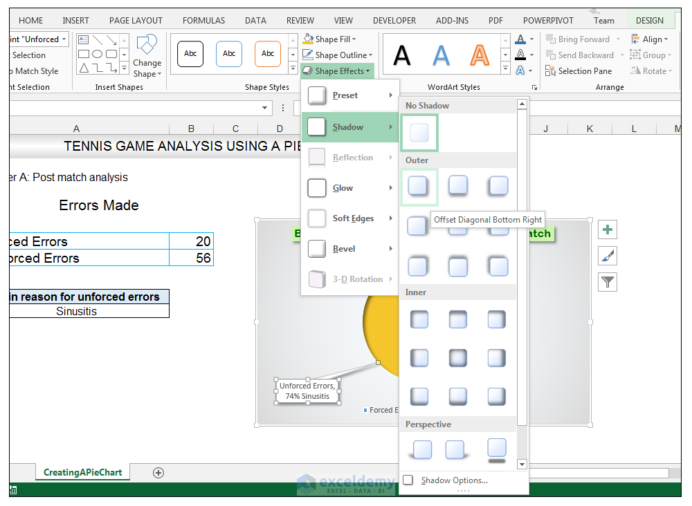
How to Make a Pie Chart in Excel & Add Rich Data Labels to The Chart!

How to show percentage in pie chart in Excel? - ExtendOffice Please do as follows to create a pie chart and show percentage in the pie slices. 1. Select the data you will create a pie chart based on, click Insert > I nsert Pie or Doughnut Chart > Pie. See screenshot: 2. Then a pie chart is created. Right click the pie chart and select Add Data Labels from the context menu. 3.

How to Make a Pie Chart in Excel & Add Rich Data Labels to The Chart!

Pie of Pie Chart in Excel - Inserting, Customizing, Formatting Inserting a Pie of Pie Chart. Let us say we have the sales of different items of a bakery. Below is the data:-. To insert a Pie of Pie chart:-. Select the data range A1:B7. Enter in the Insert Tab. Select the Pie button, in the charts group. Select Pie of Pie chart in the 2D chart section.

Pie Chart – Excel Tutorials

Add or remove data labels in a chart - support.microsoft.com Click the data series or chart. To label one data point, after clicking the series, click that data point. In the upper right corner, next to the chart, click Add Chart Element > Data Labels. To change the location, click the arrow, and choose an option. If you want to show your data label inside a text bubble shape, click Data Callout.

Pie Chart GIF Animation | Browse Examples & Animate Your Graphs

How to Rotate Pie Chart in Excel? - WallStreetMojo In the next step, change the title of the chart and add data labels to it. To rotate the pie chart, click on the chart area. Right-click on the pie chart and select the "format data series" option. Change the angle of the first scale to 90 degrees to display the chart properly.

How to Create a Pie Chart in Excel using Worksheet Data

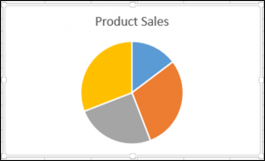
How to Create Pie Charts in Excel (In Easy Steps) 6. Create the pie chart (repeat steps 2-3). 7. Click the legend at the bottom and press Delete. 8. Select the pie chart. 9. Click the + button on the right side of the chart and click the check box next to Data Labels. 10. Click the paintbrush icon on the right side of the chart and change the color scheme of the pie chart. Result: 11.

New, better alternative to Pie Charts: Treemap - Efficiency 365

Pie Chart in Excel | How to Create Pie Chart - EDUCBA Pie Chart in Excel is used for showing the completion or main contribution of different segments out of 100%. It is like each value represents the portion of the Slice from the total complete Pie. For Example, we have 4 values A, B, C and D.

Simple Pie Chart

Excel custom pie chart labels - Microsoft Community Excel custom pie chart labels I have a data set like this (basically form output): I want to use a pivot table to make a pie chart out of this. I want each of the pieces of the pie to contain the number of entries and between parentheses the percentage. So in the "Yes" piece, there should be '3 (33%)'.

VBA Guide For Charts and Graphs - Automate Excel

Edit titles or data labels in a chart - support.microsoft.com On a chart, click the label that you want to link to a corresponding worksheet cell. On the worksheet, click in the formula bar, and then type an equal sign (=). Select the worksheet cell that contains the data or text that you want to display in your chart. You can also type the reference to the worksheet cell in the formula bar.

How to Make a Pie Chart in Excel & Add Rich Data Labels to The Chart!

Multiple data labels (in separate locations on chart) You can do it in a single chart. Create the chart so it has 2 columns of data. At first only the 1 column of data will be displayed. Move that series to the secondary axis. You can now apply different data labels to each series. Attached Files 819208.xlsx‎ (13.8 KB, 264 views) Download Cheers Andy Register To Reply

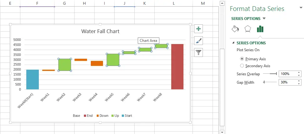
Waterfall Chart in Excel - DataScience Made Simple

Microsoft Excel Tutorials: Add Data Labels to a Pie Chart You should get the following menu: From the menu, select Add Data Labels. New data labels will then appear on your chart: The values are in percentages in Excel 2007, however. To change this, right click your chart again. From the menu, select Format Data Labels: When you click Format Data Labels , you should get a dialogue box.

Microsoft Excel Data Table - Super User

How to Make a Pie Chart in Excel & Add Rich Data Labels to The Chart! Creating and formatting the Pie Chart 1) Select the data. 2) Go to Insert> Charts> click on the drop-down arrow next to Pie Chart and under 2-D Pie, select the Pie Chart, shown below. 3) Chang the chart title to Breakdown of Errors Made During the Match, by clicking on it and typing the new title.

Creating Pie of Pie and Bar of Pie charts

excel - Positioning data labels in pie chart - Stack Overflow Positioning data labels in pie chart. I'm trying to format some charts I have, using VBA. To get started I recorded a macro of me doing what I wanted, to have an idea of what methods I'd want etc. The recorded macro looks like this - I'm including the whole thing, though the line to pay attention to is Selection.Position = xlLabelPositionCenter.

Share :