40 data labels excel chart
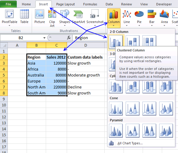
How to Customize Your Excel Pivot Chart Data Labels - dummies The Data Labels command on the Design tab's Add Chart Element menu in Excel allows you to label data markers with values from your pivot table. When you click the command button, Excel displays a menu with commands corresponding to locations for the data labels: None, Center, Left, Right, Above, and Below. None signifies that no data labels should be added to the chart and Show signifies ... Modify Excel Chart Data Range | CustomGuide The new data needs to be in cells adjacent to the existing chart data. Rename a Data Series. Charts are not completely tied to the source data. You can change the name and values of a data series without changing the data in the worksheet. Select the chart; Click the Design tab. Click the Select Data button.
Excel charts: how to move data labels to legend ... @Matt_Fischer-Daly . You can't do that, but you can show a data table below the chart instead of data labels: Click anywhere on the chart. On the Design tab of the ribbon (under Chart Tools), in the Chart Layouts group, click Add Chart Element > Data Table > With Legend Keys (or No Legend Keys if you prefer)
Data labels excel chart
How to I rotate data labels on a column chart so that they ... To change the text direction, first of all, please double click on the data label and make sure the data are selected (with a box surrounded like following image). Then on your right panel, the Format Data Labels panel should be opened. Go to Text Options > Text Box > Text direction > Rotate Adding rich data labels to charts in Excel 2013 ... The rich data label capabilities in Excel 2013 give you tools to create visuals that tell the story behind the data with maximum impact. The basics of data labels To illustrate some of the features and uses of data labels, let's first look at simple chart. How to use a macro to add labels to data points in an xy ... The labels and values must be laid out in exactly the format described in this article. (The upper-left cell does not have to be cell A1.) To attach text labels to data points in an xy (scatter) chart, follow these steps: On the worksheet that contains the sample data, select the cell range B1:C6.
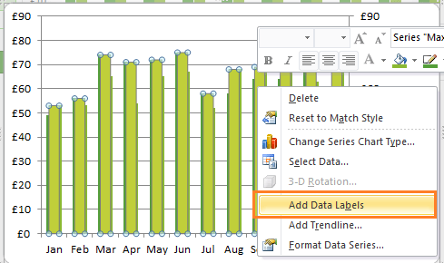
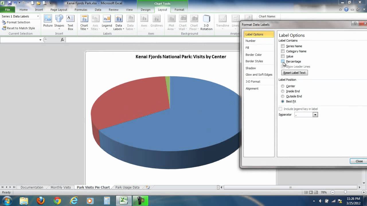
Data labels excel chart. Change the format of data labels in a chart To get there, after adding your data labels, select the data label to format, and then click Chart Elements > Data Labels > More Options. To go to the appropriate area, click one of the four icons ( Fill & Line, Effects, Size & Properties ( Layout & Properties in Outlook or Word), or Label Options) shown here. How to create a chart with both percentage and value in Excel? After installing Kutools for Excel, please do as this:. 1.Click Kutools > Charts > Category Comparison > Stacked Chart with Percentage, see screenshot:. 2.In the Stacked column chart with percentage dialog box, specify the data range, axis labels and legend series from the original data range separately, see screenshot:. 3.Then click OK button, and a prompt message is popped out to remind you ... How to create Custom Data Labels in Excel Charts Add data labels Create a simple line chart while selecting the first two columns only. Now Add Regular Data Labels. Two ways to do it. Click on the Plus sign next to the chart and choose the Data Labels option. We do NOT want the data to be shown. To customize it, click on the arrow next to Data Labels and choose More Options … How to Add Total Data Labels to the Excel Stacked Bar Chart Apr 03, 2013 · Step 4: Right click your new line chart and select “Add Data Labels” Step 5: Right click your new data labels and format them so that their label position is “Above”; also make the labels bold and increase the font size. Step 6: Right click the line, select “Format Data Series”; in the Line Color menu, select “No line” Step 7 ...
Chart.ApplyDataLabels method (Excel) | Microsoft Docs For the Chart and Series objects, True if the series has leader lines. Pass a Boolean value to enable or disable the series name for the data label. Pass a Boolean value to enable or disable the category name for the data label. Pass a Boolean value to enable or disable the value for the data label. Excel tutorial: How to use data labels Generally, the easiest way to show data labels to use the chart elements menu. When you check the box, you'll see data labels appear in the chart. If you have more than one data series, you can select a series first, then turn on data labels for that series only. You can even select a single bar, and show just one data label. Format Data Labels in Excel- Instructions - TeachUcomp, Inc. Format Data Labels in Excel: Instructions. To format data labels in Excel, choose the set of data labels to format. One way to do this is to click the "Format" tab within the "Chart Tools" contextual tab in the Ribbon. Then select the data labels to format from the "Current Selection" button group. Edit titles or data labels in a chart - support.microsoft.com On a chart, click one time or two times on the data label that you want to link to a corresponding worksheet cell. The first click selects the data labels for the whole data series, and the second click selects the individual data label. Right-click the data label, and then click Format Data Label or Format Data Labels.
Excel Charts - Aesthetic Data Labels - Tutorialspoint To place the data labels in the chart, follow the steps given below. Step 1 − Click the chart and then click chart elements. Step 2 − Select Data Labels. Click to see the options available for placing the data labels. Step 3 − Click Center to place the data labels at the center of the bubbles. Format a Single Data Label Add or remove data labels in a chart Click the data series or chart. To label one data point, after clicking the series, click that data point. In the upper right corner, next to the chart, click Add Chart Element > Data Labels. To change the location, click the arrow, and choose an option. If you want to show your data label inside a text bubble shape, click Data Callout. Add / Move Data Labels in Charts - Excel & Google Sheets ... We'll start with the same dataset that we went over in Excel to review how to add and move data labels to charts. Add and Move Data Labels in Google Sheets Double Click Chart Select Customize under Chart Editor Select Series 4. Check Data Labels 5. Select which Position to move the data labels in comparison to the bars. Excel Chart not showing SOME X-axis labels - Super User Apr 05, 2017 · In Excel 2013, select the bar graph or line chart whose axis you're trying to fix. Right click on the chart, select "Format Chart Area..." from the pop up menu. A sidebar will appear on the right side of the screen. On the sidebar, click on "CHART OPTIONS" and select "Horizontal (Category) Axis" from the drop down menu.
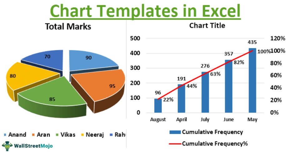
Chart Templates in Excel | 10 Steps to Create Excel Chart Template
Adding Data Labels to Your Chart (Microsoft Excel) To add data labels in Excel 2013 or Excel 2016, follow these steps: Activate the chart by clicking on it, if necessary. Make sure the Design tab of the ribbon is displayed. (This will appear when the chart is selected.) Click the Add Chart Element drop-down list. Select the Data Labels tool.
Custom data labels in a chart | Get Digital Help - Microsoft Excel resource
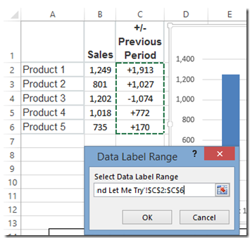
Excel Charts: Creating Custom Data Labels - YouTube In this video I'll show you how to add data labels to a chart in Excel and then change the range that the data labels are linked to. This video covers both W...
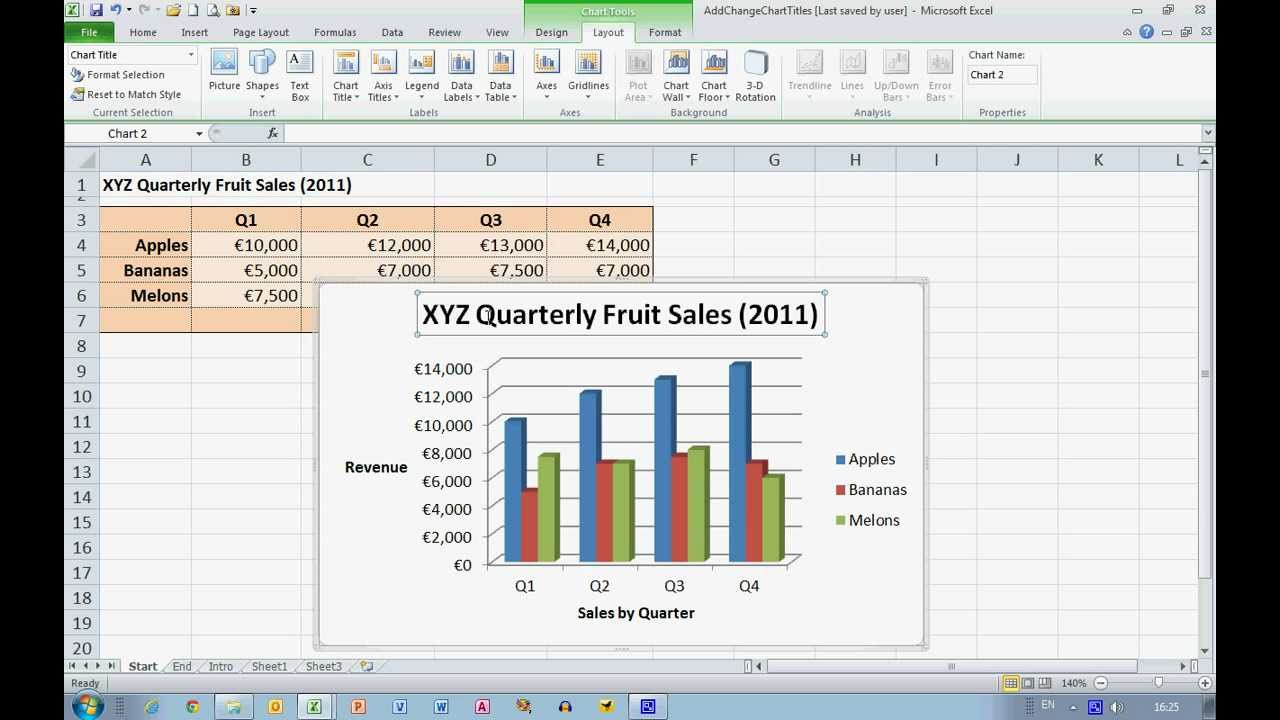
How To... Add and Change Chart Titles in Excel 2010 - YouTube
How to Add Data Labels to an Excel 2010 Chart - dummies Excel provides several options for the placement and formatting of data labels. Use the following steps to add data labels to series in a chart: Click anywhere on the chart that you want to modify. On the Chart Tools Layout tab, click the Data Labels button in the Labels group. A menu of data label placement options appears: None: The default ...
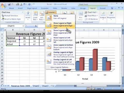
How to add or remove legends, titles or data labels in MS Excel - YouTube
How to add or move data labels in Excel chart? In Excel 2013 or 2016. 1. Click the chart to show the Chart Elements button . 2. Then click the Chart Elements, and check Data Labels, then you can click the arrow to choose an option about the data labels in the sub menu. See screenshot: In Excel 2010 or 2007. 1. click on the chart to show the Layout tab in the Chart Tools group. See ...
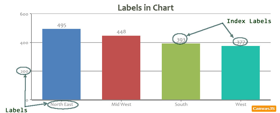
Tutorial on Labels & Index Labels in Chart | CanvasJS JavaScript Charts
Custom Chart Data Labels In Excel With Formulas Follow the steps below to create the custom data labels. Select the chart label you want to change. In the formula-bar hit = (equals), select the cell reference containing your chart label's data. In this case, the first label is in cell E2. Finally, repeat for all your chart laebls.

Chapter 3 Excel 2007/2010 Charts
Create a multi-level category chart in Excel - ExtendOffice Create a multi-level category column chart in Excel. In this section, I will show a new type of multi-level category column chart for you. As the below screenshot shown, this kind of multi-level category column chart can be more efficient to display both the main category and the subcategory labels at the same time.

How to Change Excel Chart Data Labels to Custom Values? | Chandoo.org - Learn Microsoft Excel Online
How To Use Dynamic Data Labels To Create Interactive Excel ... To create a column chart with dynamic data labels, you need to follow these given steps. Select the data & Create a Combo Chart. Now select the column chart for revenue data and a line chart with marker for data labels Add Data Labels to the Line Chart With Marker. After then remove the Line Color and Marker Color.
35 What Is Data Label In Excel - Labels For You
How to Use Cell Values for Excel Chart Labels Select the chart, choose the "Chart Elements" option, click the "Data Labels" arrow, and then "More Options." Uncheck the "Value" box and check the "Value From Cells" box. Select cells C2:C6 to use for the data label range and then click the "OK" button. The values from these cells are now used for the chart data labels.
How-to Use Data Labels from a Range in an Excel Chart - Excel Dashboard Templates
How to hide zero data labels in chart in Excel? - ExtendOffice Sometimes, you may add data labels in chart for making the data value more clearly and directly in Excel. But in some cases, there are zero data labels in the chart, and you may want to hide these zero data labels. Here I will tell you a quick way to hide the zero data labels in Excel at once. Hide zero data labels in chart
Excel Custom Chart Labels • My Online Training Hub
Move data labels - support.microsoft.com Click any data label once to select all of them, or double-click a specific data label you want to move. Right-click the selection > Chart Elements > Data Labels arrow, and select the placement option you want. Different options are available for different chart types.
Column Chart in Excel - Easy Excel Tutorial
How to add data labels from different column in an Excel chart? This method will guide you to manually add a data label from a cell of different column at a time in an Excel chart. 1.Right click the data series in the chart, and select Add Data Labels > Add Data Labels from the context menu to add data labels.
Creating a 3D Pie Chart in Excel Vid.wmv - YouTube
Add data labels to your Excel bubble charts - TechRepublic Add data labels to your Excel bubble charts . If you want to add labels to the bubbles in an Excel bubble chart, you have to do it after you create the chart. Mary Ann Richardson explains what you ...
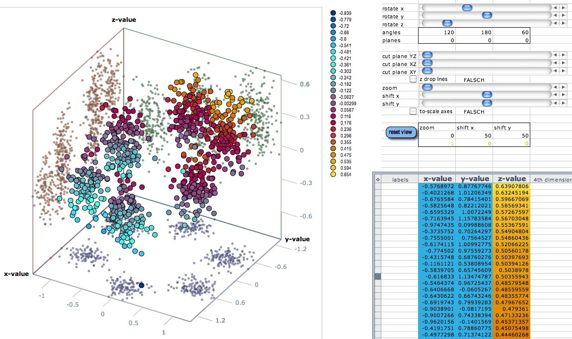
3d scatter plot for MS Excel
Change the format of data labels in a chart To get there, after adding your data labels, select the data label to format, and then click Chart Elements > Data Labels > More Options. To go to the appropriate area, click one of the four icons ( Fill & Line, Effects, Size & Properties ( Layout & Properties in Outlook or Word), or Label Options) shown here.
Making a scatter plot in Excel Mac 2011 - YouTube
How to Change Excel Chart Data Labels to Custom Values? First add data labels to the chart (Layout Ribbon > Data Labels) Define the new data label values in a bunch of cells, like this: Now, click on any data label. This will select "all" data labels. Now click once again. At this point excel will select only one data label.

How-to Use Data Labels from a Range in an Excel Chart - Excel Dashboard Templates
Custom Data Labels with Colors and Symbols in Excel Charts ... The basic idea behind custom label is to connect each data label to certain cell in the Excel worksheet and so whatever goes in that cell will appear on the chart as data label. So once a data label is connected to a cell, we apply custom number formatting on the cell and the results will show up on chart also. Following steps help you ...

Enable or Disable Excel Data Labels at the click of a button - How To - PakAccountants.com
Add a DATA LABEL to ONE POINT on a chart in Excel | Excel ... Click on the chart line to add the data point to. All the data points will be highlighted. Click again on the single point that you want to add a data label to. Right-click and select ' Add data label ' This is the key step! Right-click again on the data point itself (not the label) and select ' Format data label '.

How to Make Excel Charts More Intuitive by Adding Data Labels and Tables - Data Recovery Blog
How to use a macro to add labels to data points in an xy ... The labels and values must be laid out in exactly the format described in this article. (The upper-left cell does not have to be cell A1.) To attach text labels to data points in an xy (scatter) chart, follow these steps: On the worksheet that contains the sample data, select the cell range B1:C6.
Post a Comment for "40 data labels excel chart"